About
PolymerCpp is a small program for generating two- and three-dimensional wormlike chains (WLC), a common and relatively simple model in polymer physics. A WLC describes a semi-flexible polymer, i.e. one that is rigid over short length scales and flexible over long ones. The characteristic length scale that separates these two regimes is known as the persistence length.
PolymerCpp provides a number of Python functions that exposes the C++ routines for generating WLCs, including
- infinitesimally thin WLCs
- self-avoiding WLCs
PolymerCpp was written by Marcel Stefko and Kyle M. Douglass in the Laboratory of Experimental Biophysics for modeling DNA.
User Guide
Installation
Nix
Install PolymerCpp into your current profile:
nix-env -f PolymerCpp.nix -i '.*'
Activate an interactive shell with Python and the PolymerCpp package:
nix-shell shell.nix --pure
Chain Simulation
- Important Note: The API for PolymerCpp is unstable and may change
- in future versions.
Three dimensions (3D)
To begin, start the Python interpreter and import the function to generate wormlike chains into the session’s namespace:
>>> from PolymerCpp.helpers import getCppWLC
A single realization of an infinitesimally thin wormlike chain requires two input arguments: the chain length and the persistence length:
>>> pathLength = 500
>>> persisLength = 50
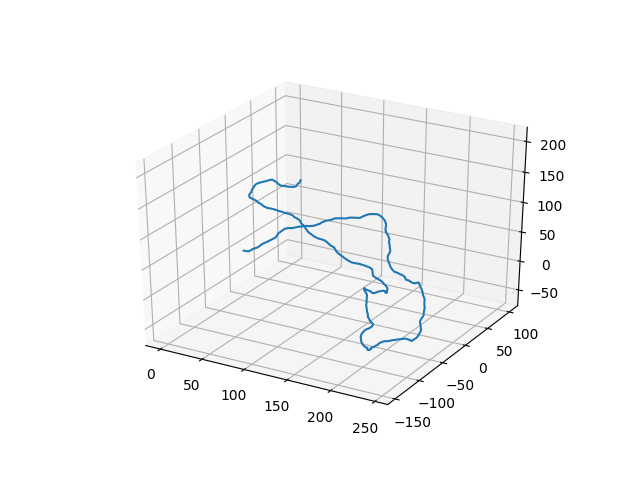
A single realization of the chain is generated by a call to getCppWLC.:
>>> chain = getCppWLC(pathLength, persisLength)
A self-avoiding WLC may also be simulated. This requires setting the diameter of the exclusion volume, which is a hard sphere centered around each chain segment. The diameter is also specified in units of chain segments and cannot exceed 1:
>>> from PolymerCpp.helpers import getCppSAWLC
>>> linkDiameter = 0.75
>>> chain = getCppSAWLC(pathLength, persisLength, linkDiameter)
Two dimensions (2D)
You can create a 2D wormlike chain as follows:
>>> from PolymerCpp.helpers import getCppWLC2D
>>> chain = getCppWLC2D(pathLength, persisLength)
The self-avoiding wormlike chain in two dimensions is not yet implemented.
Verification of the Algorithms
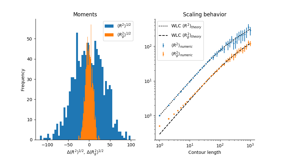
PolymerCpp.algorithms contains a utility function that performs two numerical experiments for verifying the accuracy of the algorithms. In the first, it calculates chain realizations for a given number of groups and a given number of chain realizations for each group. The mean end-to-end distance R and mean radius of gyration Rg is computed for each group and a histogram of the results is displayed. The x-axis is the difference between the computed mean and the theoretical mean.
In the second experiment, a number of chains are simulated for a range of chain contour lengths. The mean end-to-end distance and mean radius of gyration for each group is then plotted vs. the contour length, along with the theoretical predications. The error bars denote the standard deviation of the group:
from PolymerCpp.algorithms import verifyWLC
verifyWLC(getCppWLC)
This will print a summary to the console and display a figure similar to the following:
You may change a number of settings by specifying arguments to the function:
verifyWLC(getCppSAWLC,
          numChains=50,
          numExperiments=500,
          pathLength=800,
          persisLength=20,
          linkDiameter=0.5)
Bias
The bias observed in the radius of gyration at short distances is due to the fact that the chain is represented by the coordinates of the endpoints of its segments. The radius of gyration of a line of unit length is \(1 / \left( 2 \sqrt{3} \right)\), whereas the radius of gyration of a set consisting of only its endpoints is \(1 /2\).
Algorithm
Wormlike Chain
Three dimensions (3D)
The WLC algorithm is based on a discretized version of the original Kratky-Porod model of a continuous semiflexible polymer. To our knowledge, the algorithm was first described in Ref. [1] and was therein referred to as the random \(\phi\) model. In this model, the chain is approximated as a series of discrete segments of equal length. In spherical coordinates, the change in direction between successive segments is described by two angles: the zenith angle \(\theta\) and the azimuthal angle \(\phi\). The azimuthal angle is allowed to vary randomly and uniformly between \(0\) and \(2\pi\) (hence the model’s name). The zenith angle however is a random number whose probability distribution function (p.d.f.) reflects the rigidty of the polymer.
The p.d.f. for the zenith angle is derived by considering the change in local free energy due entirely to bending of the polymer between segments. (Any energy due to other forces between the segments, e.g. torsion, are ignored.) The Taylor series expansion about \(\theta_i = 0\) for the change in local free energy \(\Delta U_i \left( \theta \right)\) between segments \(i\) and \(i+1\) is
At equilibrium, the the first derivative is zero. Under this condition and ignoring all terms of third order and higher, the p.d.f. for \(\theta\) may be obtained by substituting the expansion for the local free energy change into the Boltzmann distribution \(p \left( \Delta U \right) \sim \exp \left( \frac{- \Delta U}{k_B T} \right)\)
where \(N^{-1/2}\) is a normalization constant, \(a_i = U_i''/k_B T\), and \(sin \, \theta_i\) is a weighting factor that reflects the fact that the integration over the number of possible bending angles in spherical coordinates has a differential solid angle \(d \Omega = sin \, \theta \, d \theta \, d \phi\).
Normalizing this distribution is difficult because of the presence of \(sin \, \theta_i\) in the expression above. However, if \(a_i\) is sufficiently large (i.e. the polymer is sufficiently rigid), then \(sin \, \theta_i\) may be approximated as \(\theta_i\) and the normalization is easily performed by extending the limits of integration to infinity.
The last equation is a result of integrating over the azimuthal angle from \(0\) to \(2 \pi\). Finally, assuming that \(a_i\) is the same for the bending between each segment, we arrive at a Rayleigh distribution for the zenith angle between segments.
In the simulation, the chain is created by simulating a random walk on the surface of the unit sphere. The walk begins at a predefined point on the sphere, typically the defined by the vector \(\left( 1, 0, 0 \right)\) in Cartesian coordinates. The next step of the walk is generated by selecting a random direction in the plane tangent to the sphere at that point and that is uniformly distributed between \(0\) and \(2 \pi\). The length of the displacement in this plane is calculated by taking the sine of a random variate
where \(X\) is a random variate uniformly distributed between 0 and 1. This transformation produces random numbers with a p.d.f. for \(\theta\) that is equivalent to the expression derived above.
After moving a distance \(\sin \, \theta\) in the tanget plane in the direction defined by \(\phi\), the new point is back-projected onto the sphere and defines the next point in the walk. This is repeated a pre-defined number of times and the final chain is calculated by cumulative summation over all the vectors in the walk.
According to Ref. [1], the parameter \(a\) is–to very high accuracy–equivalent to the chain’s persistence length. For this reason, we use the approximation
Strictly speaking, the persistence length of the chain in this model is
where \(L \left( a \right)\) is the Langevin function. With the equivalence \(a = \ell_p\), we now have an expression for obtaining a random number that represents the zenith angle between segments in terms of the chain’s persistence length. This is the main result of this discussion.
This algorithm generates an infinitesimally thin wormlike chain because no collision checking is performed.
Two dimensions (2D)
In two dimensions, there is no need to model rotations out of the xy plane. The probability distribution for the bending angle \(\theta\) between neighboring segments is
The chain is generated by simulating a random walk on the unit circle. Starting from a unit vector in the xy plane, the next segment of the chain is generated by rotating this initial vector about the z-axis by an angle that is a random variate whose probability distribution is given by the above expression. Each successive segment is computed by rotating the current segment by such a random angle, and the final chain is constructed by a cumulative summation of all vectors that were generated during the walk.
Self-avoiding wormlike chain
The self-avoiding WLC is modeled a series of spheres whose center-to-center distances is fixed for successive spheres. The zenith angle between the segments joining successive spheres is determined in the same manner as described for the wormlike chain. For each successive sphere, a candidate sphere is generated and checked for collisions with other spheres in the chain. If there is a collision, the sphere is erased and another sphere is generated.
Indices and tables
Footnotes
| [1] | (1, 2) Schellman, J. A., “Flexibility of DNA,” Biopolymers 13, 217-226 (1974). |